Here we are sharing the experiences of the natESM Research Software Engineers (RSE) that have been gathered during individual sprints or when dealing with specific HPC environments. Additionally, the RSE are providing solutions to coding challenges for your benefit.
User-Defined Derived Type Input/Output with NVHPC compiler
Author: Enrico Degregori (formerly DKRZ)
User-Defined Derived Type Input/Output (UDTIO) allows the programmer to specify how a derived type is read or written from or to a file. This allows the user of an object to perform Input/Output operations without any knowledge of the object's layout.
Case study: Unformatted I/O
Consider the following mesh class:
type t_meshinteger :: nod2Dreal(kind=WP) :: ocean_areareal(kind=WP), allocatable, dimension(:,:) :: coord_nod2Dcontainsprocedure, private write_t_meshprocedure, private read_t_meshgeneric :: write(unformatted) => write_t_meshgeneric :: read(unformatted) => read_t_meshend type t_mesh
The subroutines for IO of this derived data type are:
subroutine write_t_mesh(mesh, unit, iostat, iomsg)
class(t_mesh), intent(in) :: meshinteger, intent(in) :: unitinteger, intent(out) :: iostatcharacter(*), intent(inout) :: iomsg
write(unit, iostat=iostat, iomsg=iomsg) mesh%nod2Dwrite(unit, iostat=iostat, iomsg=iomsg) mesh%ocean_areacall write_bin_array(mesh%coord_nod2D, unit, iostat, iomsg)
end subroutine write_t_mesh
subroutine read_t_mesh(mesh, unit, iostat, iomsg)
class(t_mesh), intent(inout) :: meshinteger, intent(in) :: unitinteger, intent(out) :: iostatcharacter(*), intent(inout) :: iomsg
read(unit, iostat=iostat, iomsg=iomsg) mesh%nod2Dread(unit, iostat=iostat, iomsg=iomsg) mesh%ocean_areacall read_bin_array(mesh%coord_nod2D, unit, iostat, iomsg)
end subroutine read_t_mesh
In the main program then the object can be read/written without knowing the derived data type layout:
program main
implicit nonetype(t_mesh) :: mesh
! mesh derived typeopen(newunit = fileunit, & file = trim(path_in), & status = 'replace', & form = 'unformatted')write(fileunit) meshclose(fileunit)
end program main
NVHPC compiler requires the writing/reading subroutines to be defined as private. If also the generic write/read are defined as private, the program will note fail with a runtime error but inconsistent behaviors can be observed (like wrong data read from files).
Compilation errors
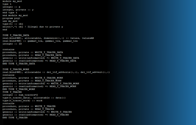
Private components of a derived data type are not accessible with traditional IO operations, so the following code generates a compilation error:
module my_modtype t integer :: x integer, private :: yend type tend module my_modprogram prg1use my_modtype(t) :: objwrite(*,*) obj ! Illegal due to private yend
F2003 also does not allow IO operations on entire objects that have pointer components, so the following code generates a compilation error:
module my_modtype t integer :: x integer,pointer :: yend typeend module my_modprogram prg2use my_modtype(t) :: objwrite(*,*) obj ! Illegal due to pointer yend
If a derived data type contains an allocatable array of another derived data type, the UDTIO operation fails at compile time. For example:
TYPE T_TRACER_DATAreal(kind=WP), allocatable, dimension(:,:) :: values, valuesABreal(kind=WP) :: gamma0_tra, gamma1_tra, gamma2_trainteger :: ID
containsprocedure, private :: WRITE_T_TRACER_DATAprocedure, private :: READ_T_TRACER_DATAgeneric :: write(unformatted) => WRITE_T_TRACER_DATAgeneric :: read(unformatted) => READ_T_TRACER_DATAEND TYPE T_TRACER_DATA
TYPE T_TRACER_WORKreal(kind=WP), allocatable :: del_ttf_advhoriz(:,:), del_ttf_advvert(:,:)
containsprocedure, private :: WRITE_T_TRACER_WORKprocedure, private :: READ_T_TRACER_WORKgeneric :: write(unformatted) => WRITE_T_TRACER_WORKgeneric :: read(unformatted) => READ_T_TRACER_WORKEND TYPE T_TRACER_WORK
TYPE T_TRACERinteger :: num_tracers=2type(t_tracer_data), allocatable :: data(:)type(t_tracer_work) :: workcontainsprocedure, private :: WRITE_T_TRACERprocedure, private :: READ_T_TRACERgeneric :: write(unformatted) => WRITE_T_TRACERgeneric :: read(unformatted) => READ_T_TRACEREND TYPE T_TRACER
Debugging during GPU porting with OpenACC
Author: Enrico Degregori (formerly DKRZ)
Parallel Compiler Assisted Software Testing (PCAST) is a feature available in the NVIDIA HPC Fortran, C++, and C compilers. It compares the GPU computation against the same program running on the CPU. In this case, all compute constructs are done redundantly, on both CPU and GPU. The GPU results can then be compared against the CPU results and the differences reported.
A semi-automatic method which can be used with OpenACC is to allow the runtime to automatically compare values when they are downloaded from device memory. This is enabled with the -gpu=autocompare compiler flag, which also enables the redundant option. This runs each compute construct redundantly on CPU and GPU and compares the results, with no changes to the program itself.
The autocompare feature only compares data when it would get downloaded to system memory. To compare data after some compute construct that is in a data region, where the data is already present on the device, there are three ways to do the comparison at any point in the program.
-
First, you can insert an
update selfdirective to download the data to compare. With the autocompare option enabled, any data downloaded with anupdate selfdirective will be downloaded from the GPU and compared to the values computed on the host CPU. -
Alternatively, you can add a call to
acc_compare, which compares the values then present on the GPU with the corresponding values in host memory. Theacc_compareroutine has only two arguments: the address of the data to be compared and the number of elements to compare. The data type is available in the OpenACC runtime, so doesn’t need to be specified.
Finally, you can use the acc compare directive.
Autocompare is useful to debug differences between CPU and GPU results during the porting. When during the porting the developer is facing a runtime error, the NVHPC compiler is often not giving much information. In this case, it is useful to set export NVCOMPILER_ACC_NOTIFY=3 in the batch script to get useful information about data movements and kernel launching in order to locate the part of the code responsible for the crash.
Port and enable HIP as a Kokkos backend of the ParFlow model using eDSL
Author: Jörg Benke (JSC)
The main idea of the ParFlow sprint was to port and to enable HIP as a Kokkos backend of the hydrologic model ParFlow using the eDSL (embedded Domain Specific Language) of ParFlow. The usage of the eDSL and Kokkos allows in principle a very easy adaptation to different architectures and parallel models. This was the case when porting ParFlow to CUDA with Kokkos. We will shortly list a few points what we have learnt in this sprint regarding the porting efforts for HIP and Kokkos.
- Kokkos v4.0 breaks backwards compatibility with Kokkos v3.7 for AMD support. The update to Kokkos v4.0 required some updates in the Kokkos API in ParFlow.
- The response time of the support for Kokkos via its slack channel is very quick.
- Using the different tools of the Kokkos ecosystem (e.g., kernel logger of Kokkos) or AMD debugging/logging flags in ParFlow (export AMD_LOG_LEVEL=4) are in general very helpful for logging and debugging.
- HIPification via eDSL and Kokkos is in principle relatively easy. We’ve modified the ParFlow eDSL to enable the Kokkos API to reach the HIP backend, mimicking the approach already enabled for CUDA.
- Compiling ParFlow with the HIPFortran of the ROCm environment was challenging because compilation with the standard installed HIPFortran wasn’t possible. This was the case also on LUMI-G, we circumvented it with cloning HIP Fortran and compiling it on our own.
Modular Supercomputing Architecture (MSA) concept at JSC
Author: Catrin Meyer (JSC)
The Modular Supercomputing Architecture concept is a novel way of organizing computing resources in HPC systems, developed at the Jülich Supercomputing Centre (JSC) in the course of the DEEP projects. Its key idea is to segregate hardware resources (e.g. CPUs, GPUs, other accelerators) into separate modules such that the nodes within each module are maximally homogeneous. This approach has the potential to bring substantial benefits for heterogeneous applications, wherein each sub-component has been tailored or is by nature of the numerical solution better suited to run efficiently on specific hardware.
General commands to perform heterogeneous simulations on the Jülich HPC systems
Submission commands
- Multiple independent job specifications identified in command line separated by “:”.
salloc <options 0 + common> : <options 1> [ : <options 2>... ]
- Resulting heterogeneous job will have as many job components as there were blocks of command line arguments
- The first block of arguments contains the job options of the first job component as well as common job options that will apply to all other components. The second block contains options for the second job component and so on.
- Example:
salloc -A budget -p partition_a -N 1 : -p partition_b -N 16
- Submitting non-interactive heterogeneous jobs through sbatch works similarly, but the syntax for seperating blocks of options in a batch script is slightly different.
- Use
#SBATCH hetjobbetween the other#SBATCHoptions in jobscript to separate job packs and their groups of resources. - With srun and the “:” format you can spawn jobsteps using heterogeneous resources.
- With the srun’s option --het-group you can define which het-group of resources will be used for the jobsteps.
srun <options and command 0> : <options and command 1> [ : <options and command 2> ]- The first block applies to the first component, the second block to the second component and so on. If there are less blocks than job components, the resources of the latter job components go unused as no application is launched there.
- The option
--het-group=<expr>can be used to explicitly assign a block of command line arguments to a job component. It takes as its argument<expr>either a single job component index in the range 0 ... n - 1 where n is the number of job components, or a range of indices like 1-3 or a comma seperated list of both indices and ranges like 1,3-5.
Example of a jobscript
#!/bin/bash
#SBATCH -N 32 --ntasks-per-node=8 -p batch
#SBATCH hetjob
#SBATCH -N 1 --ntasks-per-node=1 -p batch
#SBATCH hetjob
#SBATCH -N 16 --gres=gpu:4--ntasks-per-node=4 -p gpus
srun --het-group=0 exec0 : --het-group=1 exec1 : --het-group=2 exec2
Example of a scientific use case
The ICON model was ported to and optimized on the MSA-system Jülich Wizard for European Leadership Science (JUWELS) at Jülich Supercomputing Centre, in such a manner that the atmosphere component of ICON runs on GPU equipped nodes, while the ocean component runs on standard CPU-only nodes. Both, atmosphere and ocean, are running globally with a resolution of 5 km. In our test case, an optimal configuration in terms of model performance (core hours per simulation day) was found for the combination 84 GPU nodes on the JUWELS Booster module and 80 CPU nodes on the JUWELS Cluster module, of which 63 nodes were used for the ocean simulation and the remaining 17 nodes were reserved for I/O. With this configuration the waiting times of the coupler were minimized. Compared to a simulation performed on CPUs only, the energy consumption of the MSA approach was nearly halved with comparable runtimes.
More details can be found in: Bishnoi, A., Stein, O., Meyer, C. I., Redler, R., Eicker, N., Haak, H., Hoffmann, L., Klocke, D., Kornblueh, L., and Suarez, E.: Earth system modeling on Modular Supercomputing Architectures: coupled atmosphere-ocean simulations with ICON 2.6.6-rc, EGUsphere [preprint],
https://doi.org/10.5194/egusphere-2023-1476, 2023.
Poor implementation of OpenACC PRIVATE clause in the NVHPC compiler
Author: Enrico Degregori (formerly DKRZ)
A single column component of a climate model is characterized by dependencies in the vertical coordinate. In this case it is usual to allocate a temporary array which is used on every iteration over the surface points. An example with ICON data structures:
!ICON_OMP_PARALLEL_DO PRIVATE(startIndex, endIndex) ICON_OMP_DEFAULT_SCHEDULEDO jb = cells_in_domain%start_block, cells_in_domain%end_block CALL get_index_range(cells_in_domain, jb, startIndex, endIndex) DO jc = start_index, end_index levels = dolic_c(jc,jb) IF (dolic_c(jc,jb) > 0) THEN DO level = 1, levels pressure(level) = fill_pressure_ocean_physics() END DO DO level = 1, levels-1 rho_up(level) = calculate_density(& & temp(jc,level,jb), & & salt(jc,level,jb), & & pressure(level+1)) END DO DO level = 2, levels rho_down(level) = calculate_density(& & temp(jc,level,jb), & & salt(jc,level,jb), & & pressure(level)) END DO DO level = 2, levels Nsqr(jc,level,jb) = gravConstant * (rho_down(level) - rho_up(level-1)) * & dzi(jc,level,jb) / s_c(jc,jb) END DO END IF END DOEND DO ! end loop over blocks!ICON_OMP_END_PARALLEL_DO
A possible way to port this short example is to parallelize over the jc loop given that the range start_index:end_index is large enough to fill the GPU.
!ICON_OMP_PARALLEL_DO PRIVATE(startIndex, endIndex) ICON_OMP_DEFAULT_SCHEDULEDO jb = cells_in_domain%start_block, cells_in_domain%end_block CALL get_index_range(cells_in_domain, jb, startIndex, endIndex) !$ACC PARALLEL LOOP GANG VECTOR PRIVATE(rho_up, rho_down, pressure) DEFAULT(PRESENT) DO jc = start_index, end_index levels = dolic_c(jc,jb) IF (dolic_c(jc,jb) > 0) THEN DO level = 1, levels pressure(level) = fill_pressure_ocean_physics() END DO DO level = 1, levels-1 rho_up(level) = calculate_density(& & temp(jc,level,jb), & & salt(jc,level,jb), & & pressure(level+1)) END DO DO level = 2, levels rho_down(level) = calculate_density(& & temp(jc,level,jb), & & salt(jc,level,jb), & & pressure(level)) END DO DO level = 2, levels Nsqr(jc,level,jb) = gravConstant * (rho_down(level) - rho_up(level-1)) * & dzi(jc,level,jb) / s_c(jc,jb) END DO END IF END DO !$ACC END PARALLEL LOOPEND DO ! end loop over blocks!ICON_OMP_END_PARALLEL_DO
This parallelization strategy allows to have memory coalescing and, assuming that the horizontal resolution is high enough, maximal throughput can be achieved. However, when profiling the kernel (using Nsight Systems or Nsight Compute), the performance is poor and the occupancy is quite low because of a high utilization of registers. The reason is that the compiler is not allocating the PRIVATE variables in global memory and since their size is equal to the number of vertical levels, the register utilization increases and as a consequence the occupancy decreases.
A possible workaround (purely for GPU performance) is to extend the dimension of the temporary variables, so that they don't have to be PRIVATE and can be allocated in global memory:
!ICON_OMP_PARALLEL_DO PRIVATE(startIndex, endIndex) ICON_OMP_DEFAULT_SCHEDULE
DO jb = cells_in_domain%start_block, cells_in_domain%end_block
    CALL get_index_range(cells_in_domain, jb, startIndex, endIndex)
    !$ACC PARALLEL LOOP GANG VECTOR DEFAULT(PRESENT)
    DO jc = start_index, end_index
        levels = dolic_c(jc,jb)
        IF (dolic_c(jc,jb) > 0) THEN
            DO level = 1, levels
                pressure(jc,level) = fill_pressure_ocean_physics()
            END DO
            DO level = 1, levels-1
                rho_up(jc,level) = calculate_density(&
                              & temp(jc,level,jb), &
                              & salt(jc,level,jb), &
                              & pressure(jc,level+1))
            END DO
            DO level = 2, levels
                rho_down(jc,level) = calculate_density(&
                                & temp(jc,level,jb), &
                                & salt(jc,level,jb), &
                                & pressure(jc,level))
            END DO
            DO level = 2, levels
                Nsqr(jc,level,jb) = gravConstant * (rho_down(jc,level) - rho_up(jc,level-1)) * &
                                    dzi(jc,level,jb) / s_c(jc,jb)
            END DO
        END IF
    END DO
    !$ACC END PARALLEL LOOP
END DO ! end loop over blocks
!ICON_OMP_END_PARALLEL_DO
The performance of the kernel shows now a significant improvement but it is still suboptimal because the memory access of rho_up, rho_down and pressure is not coalesced. As a result, it would be necessary to fully restructure the loops until this compiler bug will be fixed.
GPU porting towards throughput or time-to-solution
Author: Enrico Degregori (formerly DKRZ)
When porting a code to GPU, two different approaches are possible: achieve maximum throughput or minimum time-to-solution. Let's consider a simple example based on ICON data structure:
!ICON_OMP_PARALLEL_DO PRIVATE(startIndex, endIndex) ICON_OMP_DEFAULT_SCHEDULEDO jb = cells_in_domain%start_block, cells_in_domain%end_block CALL get_index_range(cells_in_domain, jb, startIndex, endIndex) DO jc = start_index, end_index levels = dolic_c(jc,jb) IF (dolic_c(jc,jb) > 0) THEN DO level = 1, levels Nsqr(jc,level,jb) = gravConstant * (rho_down(jc,level,jb) - rho_up(jc,level-1,jb)) * & dzi(jc,level,jb) END DO END IF END DOEND DO ! end loop over blocks!ICON_OMP_END_PARALLEL_DO
GPU porting towards maximum throughput would look like this:
!ICON_OMP_PARALLEL_DO PRIVATE(startIndex, endIndex) ICON_OMP_DEFAULT_SCHEDULEDO jb = cells_in_domain%start_block, cells_in_domain%end_block CALL get_index_range(cells_in_domain, jb, startIndex, endIndex) !$ACC PARALLEL LOOP GANG VECTOR DEFAULT(PRESENT) DO jc = start_index, end_index levels = dolic_c(jc,jb) IF (dolic_c(jc,jb) > 0) THEN DO level = 1,levels Nsqr(jc,level,jb) = gravConstant * (rho_down(jc,level,jb) - rho_up(jc,level-1,jb)) * & dzi(jc,level,jb) END DO END IF END DO !$ACC END PARALLEL LOOPEND DO ! end loop over blocks!ICON_OMP_END_PARALLEL_DO
While towards minimum time-to-solution:
!ICON_OMP_PARALLEL_DO PRIVATE(startIndex, endIndex) ICON_OMP_DEFAULT_SCHEDULEDO jb = cells_in_domain%start_block, cells_in_domain%end_block CALL get_index_range(cells_in_domain, jb, startIndex, endIndex) max_levels = maxval(dolic_c(start_index:end_index,jb)) !$ACC PARALLEL LOOP GANG VECTOR COLLAPSE(2) DEFAULT(PRESENT) DO level = 1, max_levels DO jc = start_index, end_index IF (dolic_c(jc,jb) > 0 .AND. level <= dolic_c(jc,jb)) THEN Nsqr(jc,level,jb) = gravConstant * (rho_down(jc,level,jb) - rho_up(jc,level-1,jb)) * & dzi(jc,level,jb) END IF END DO END DO !$ACC END PARALLEL LOOPEND DO ! end loop over blocks!ICON_OMP_END_PARALLEL_DO
In both cases the memory access is coalesced, but the main difference is the work done by each thread.
- In the first case, the maximum number of threads executing in parallel is equal to the number of surface cells and each thread is computing the operation for each vertical level.
- In the second case, the maximum number of threads executing in parallel is equal to the total number of cells in the full domain and each thread is computing the operation once.
In an high resolution experiment, if the total number of cells on the surface are enough to use all the SMs on a GPU, the first case would have the maximum throughput. However, if we want to scale this setup to decrease the time-to-solution, the amount of work for each GPU would decrease and the second case would allow to achieve the minimum time-to-solution (better scaling).
Use of Dask´s lazy arrays instead of NumPy arrays
Author: Jörg Benke (JSC)
To optimize the memory usage of common preprocessing tasks, take advantage of out-of-core computation using Dask’s lazy arrays instead of NumPy arrays (see https://docs.dask.org/en/stable/array.html for Dask arrays), i.e., all operations are performed on smaller chunks of data rather than the entire input data at once. This avoids loading of too large data arrays into memory (“eager evaluation”), but instead works with chunks that fit comfortably into memory (“lazy evaluation”). Thus, this method enables the computation of arrays that are larger than the available memory. The idea to make the preprocessors of ESMValTool lazy and therefore more memory efficient with Dask, in addition to the already extensively used Iris library, is a valid and good approach. Its successful implementation was shown in the ported preprocessors which led to a significant improvement of memory usage and runtime. Regarding the runtime this is shown in figure 1.

Often the Dask library has a 1 to 1 mapping to the NumPy functions. In those cases the porting to Dask is often only a textual substitution of the NumPy functions like in the following example from ESMValTool
import dask.array as da
import iris

import numpy as np

...

def mask_above_threshold(cube, threshold):

"""Mask above a specific threshold value.
Takes a value 'threshold' and masks off anything that is above it in the cube data. Values equal to the threshold are not masked.
    Parameters

    ----------

    cube: iris.cube.Cube

iris cube to be thresholded.

    threshold: float
        threshold to be applied on input cube data.


Returns

-------

iris.cube.Cube

thresholded cube.

"""


(*)  cube.data = (da.ma.masked_where(cube.core_data() > threshold, cube.core_data()))
    return cube
In this function every data value of the data structure cube will be masked out which is larger than a given threshold. In line (*) two modifications had to be done. First the substitution of np (numpy) with da (dask.array). The second one was cube.data to to cube.core_data() to prevent the Iris library function to immediately realize the data. But not all NumPy functions have a 1 to 1 mapping to Dask functions which then leads to a rewriting of the code which was sometimes time consuming because the contents has to be rewritten with the help of some other Dask functions. Since the work on Dask is ongoing this gap will be probably closed for most of the NumPy functions.
Dependency tracking for linear stable Git history
Author: Wilton Loch (DKRZ)
In rapidly evolving technical contexts, like the scientific computing environment commonly is, developers usually have to keep track and update dependencies in relative high frequency. This requirement is aggravated specially when dealing with dependencies still in early development phases, where lots of changes can be expected in short periods of time.
During the MESSy-ComIn sprint this was the scenario in place. In the initial phases, due to uncertainty with regards to what would be the long term solution to keep track of ComIn, it was decided that it would be treated as a completely external library and not included directly in the MESSy project as a subtree or submodule.
Although this provided greater flexibility, it also had the negative side effect that during the development of the prototype ComIn plugin for MESSy, the ComIn version employed for each step was not tracked. Therefore, most of the commits dedicated to the implementation of this feature now represent non-stable and non-buildable states of the code, as they use a past version of the ComIn interface which is not easily recoverable.
As best practice for software management, a linear, stable, and continuously integrated (also ideally continuously deliverable) history is recommended. To reach these goals, tracking of fast moving dependencies is very important, and to projects facing a similar scenario, tracking dependencies as subtrees or ideally submodules is recommended.
Experiments with a Domain Specific Language for performance portability in Fortran
Author: Wilton Loch (DKRZ)
It is common place that codes which are tailored for better performance on CPUs do not perform the best on GPUs. This performance portability problem is well known and there are many tools and techniques that can be employed to attenuate this undesired effect. One of such solutions is reccuring to a Domain Specific Language (DSL).
A DSL can be used to create an abstraction layer which separates lower level implementation from higher level computational semantics. This allows the application to use a single front end with varied types of loops and iterative structures, which are then implemented by one or more back ends tailored to different targets, devices or infrastructures.
A proof-of-concept was devised for FESOM and employed compiler macros to create a frontend which defines n-dimensional computational spaces (e.g. operate over edges and vertical levels) and operation ranges (e.g. perform work in an n-dimensional subdomain of the computational space). The backends would then change the order of the loops in compilation time depending on whether the build target would be the CPU or GPU. The code then can look like the following:
!$ACC PARALLEL LOOP GANG VECTOR COLLAPSE(2) DEFAULT(PRESENT)

DO_NODES_AND_VERTICAL_LEVELS(node, 1, myDim_nod2D, vertical_level, 1, nl)
nzmax = nlevels_nod2D(node)

nzmin = ulevels_nod2D(node)


    OPERATE_AT(vertical_level, nzmax)

flux(vertical_level, node) = 0.0_WP - flux(vertical_level, node)

END_OPERATE_AT


OPERATE_ON_RANGE(vertical_level, nzmin + 2, nzmax - 2)

        qc = ( ttf   (vertical_level - 1, node) - ttf   (vertical_level,     node) ) &
           / ( Z_3d_n(vertical_level - 1, node) - Z_3d_n(vertical_level,     node) )

qu = ( ttf   (vertical_level,     node) - ttf   (vertical_level + 1, node) ) &
           / ( Z_3d_n(vertical_level,     node) - Z_3d_n(vertical_level + 1, node) )

qd = ( ttf   (vertical_level - 2, node) - ttf   (vertical_level - 1, node) ) &
           / ( Z_3d_n(vertical_level - 2, node) - Z_3d_n(vertical_level - 1, node) )

END_OPERATE_RANGE

END_NODES_AND_VERTICAL_LEVELS

!$ACC END PARALLEL LOOP
An experimental performance analysis test was done with the FESOM QR4C kernel, and results are shown in the following plot:

The DSL approach is able to attain near optimal performance for both targets with one single codebase. Despite these very promising results in terms of performance portability, there are a number of drawbacks, related mostly to the lack of solid macro support in Fortran:
- Larger obfuscation of the code: The use of higher level and more abstract macros to define the loops may turn the code more difficult to read for some users.
- Complications due to weak Fortran support for macros:
- In order to define multiple line macros one must use semi-colons to divide the lines. Once the text substitution happens and the compilation proceeds all these lines are treated as one, which makes it harder to interpret compile-time errors and warnings.
- Less support for extended macro functions for parameter substitution and checking.
- The problem is aggravated when different compilers and compiler versions have different types of completeness for macro functionalities.
- Not straightforward to have code blocks as parameters for macros as is possible in C/C++
In this specific case of a macro-based performance DSL for Fortran, the listed drawbacks in terms of software quality are normally considered too great to pay off even with the performance benefits. This is aggravated when considering the rapid development of other more robust performance portability tools like OpenMP and even OpenACC itself.
OpenACC multicore CPU performance experiments
Author: Wilton Loch (DKRZ)
OpenACC is often used in the ESM community as a tool for porting Fortran applications to GPU. ICON is perhaps the most recognizable example, as its large atmosphere component is actively executed on GPUs for production runs on multiple computing centers. A similar OpenACC port for the ICON ocean component is also under active development.
OpenACC however, is not restricted to GPUs and is also able to target code generation for multicore CPU targets. In spite of that, no known production setups are using OpenACC as a tool for multicore CPU parallelization. During the FESOM GPU porting sprint this point came up and a small performance evaluation of the OpenACC CPU performance was made and compared against the performance of OpenMP for the same target. The results in execution time for a selected number of FESOM 2.1 kernels both with nested and collapsed loops can be seen in the following plot:

The experiments were performed in the JUWELS Cluster and for this particular setup it can be seen that for all kernels both OpenMP and OpenACC performances are generally comparable.
We also investigated the perfomance difference for more specific cases when the code requires critical regions, where atomic writes or updates are required. The following two plots show the time differences between OpenMP and OpenACC for one of the FCT kernels in FESOM 2.1 which has a critical region:


For the nested loop version OpenMP performs better, and for the collapsed version OpenACC performs better.
From these basic experiments, the OpenACC multicore CPU performance is shown to be consistent with the OpenMP performance and its production use for this target could be feasible. More comprehensive tests should be performed for more solid conclusions with focus on ESM applications. For developers considering both OpenMP and OpenACC as options for GPU and CPU parallelization a number of other factors should also be taken into account, like vendor and compiler support, additional development tools, developer community adoption, among others.
Considerations in creating ComIn plugins out of complex models for MESSy
Author: Wilton Loch (DKRZ)
The following points gather recommendations and aspects to keep in mind when creating a ComIn plugin for your model. They are drawn from the experiences gathered in the MESSy-ComIn sprints. Given the broad technical documentation on how to use ComIn provided by the ComIn developers here and reports focused on the technical aspects for MESSy-ComIn here, the following points will not focus on either. In a nutshell, the steps you have to perform in order to successfully create a ComIn plugin are listed on our Gitlab-Wiki.
Porting QUNICY subroutines (queued tasks) to GPU
Author: Sergey Sukov (JSC - FZ Jülich)
A certain approach was established during the QUINCY sprint. QUINCY subroutines are read in one after the other and compared with each other after.
The exact step-by-step sequence of how subroutines are ported to GPU can be found in this PDF.
mo_acc_util subroutine module
Author: Sergey Sukov (JSC - FZ Jülich)
Module mo_acc_utils contains a set of subroutines for comparing the real (single or double precision) values of 1D-5D matrix elements on CPU and GPU using OpenACC features. Here is a User Guide how to use it.
How to install YAC with python bindings on Levante
Author: Aleksandar Mitic (DKRZ)
This User Guide provides comprehensive tests to validate your YAC Python environment setup and installation on the Levante HPC system.
OpenACC extended porting guide
Author: Wilton Jaciel Loch (DKRZ)
An advanced companion to the official OpenACC Programming and Best Practices Guide — offering additional tips, steps, and lessons learned to make the porting process more efficient and less error-prone on HPC systems.
Read the guide on natESM GitLab.
Always consider Lag while defining fields in ICON for YAC coupling
Author: Aparna Deluvapalli (DKRZ)
Lag is a concept in YAC coupling which allows the user to manipulate the field_date_time associated with the fields set for exchange through YAC.
ICON always exchanges data from its first time step instead of the zeroth time step when the simulation starts. For this reason, we have to introduce a lag in ICON’s field definitions to recognize its first time step as the first valid “put/get”.
There are a few distinct terminologies which are important to understand before we jump into formulae associated with valid “put/get” in YAC.
start_date_time- Time at which simulation startscoupling_timestep- Frequency set by the user at which coupling needs to happenfield_time_step- Frequency set by the user to increment thefield_date_timefield_date_time- A YAC internal timer associated with fields, which gets incremented based onfield_time_step
Let us now look at ICON’s example and how YAC interprets the date and time associated with fields.
Valid put/get condition becomes true when the following becomes true.
(field_date_time - start_date_time ) % coupling_timestep == 0
Date and time associated with fields are calculated as per following equation
field_date_time = start_date_time + (lag * field_timestep)
If lag = 0 , field_date_time = start_date_time [❌]
If lag = 1 , field_date_time = start_date_time + field_timestep [✅]
Therefore, it is necessary to consider Lag while defining fields in ICON.